CHAPTER 3
Chapter 3 - The Mathematical function and its Graph
Section 3.6 - The Graph of a Function
When the independent dimension is free to take on any
value, the dependent dimension will depend on what that value is. As the
independent dimension changes, the
dependent dimension will change accordingly.
For example the function for the total kinetic energy (energy of motion)
of a moving object is expressed in terms of its mass and velocity

Using a constant mass of 4
kg, the function reduces to the following two-dimensional function.

The total energy of the body is now entirely dependent
only on the square of its velocity, whatever it may be. If the velocity were 1
m/s, the energy would be 2 Joules. If it were 2 m/s, the energy would be 8
Joules. As the velocity of the body increases, its kinetic energy also
increases. This makes sense, since the faster a body is moving, the more energy
it has.
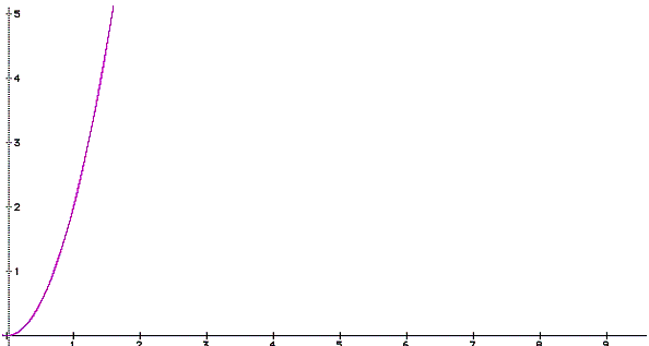
The way to visualize the changing relationship between the independent and dependent
dimension is by graphing the function on a set of perpendicular axes. The
horizontal axis is labeled after the independent dimension (condition), while
the vertical axis is labeled after the dependent dimension (situation). The graph of a function is a continuous line
that reflect a horizontal change in the independent dimension with a vertical
change in the dependent dimension. Each point on the graph represent a unique
situation . The graph of the function
 would be:
It is, however, not obvious as to how the graph of a
function is a well-defined continuous line through all the points at which the
function exists. To better understand the important relationship between a
function and its graph, consider a hypothetical function
 . In
this function, f represents an imaginary situation dependent on some condition
x. Therefore x, is our independent dimension, while f is our dependent
dimension.
For the next few chapters we will only be studying
abstract f’s and x’s. This will allow our study of the mathematical function to
be more specialized by avoiding the
confusion that arises from dealing with so many, F’s, m’s, a’s, l’s, E’s etc.
It is difficult for the mind to keep track of so many abbreviations, much
less understand where they were derived
from.

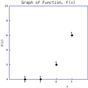
With intervals of 1
the difference between each evaluated point of our independent dimension x is 1. This gives a fairly generalized idea
of how the dependent dimension, f, changes. From x=0 to x=1, observe that f is
zero at both these points. The conclusion is that the functions value is
approximately zero from x=0 to x=1. After x=1 notice that f gets substantially larger, particularly
between x=2 and x=3. This leads to the observation that as x increases f gets
larger and larger.
Also notice that over each sub-interval the net change in
y is different.
From x=0 to x=1, f goes from
0 to 0 or the net change in f is 0
From x=1 to x=2, f goes from
0 to 2 or the net change in f is 2
From x=2 to x=3, f goes from
2 to 6 or the net change in f is 6 - 2 = 4
In each case the change in x is 1 but the corresponding change in f increases as x
increases.
Until now our discussion of the function
 has been limited to just four points, x=
0,1,2, and 3. The concept to understand is that a function is defined at every
point and the continuous line connecting the points corresponds to the graph of
the function. In order to gain a better understanding of the function, it needs
to be analyzed at more points.
Though before continuing, an important symbol will be
introduced, the Greek letter Delta,
 .
.
 is a symbol for a quantifiable change, not
metaphorically speaking! It represents a definite difference or change between
two values. For example if x changed from 8 to 21, instead of saying the change
in x is 21-8 or 13, it is more accurate to say
 x is
13 or
  x = 13 .
This symbol will be used throughout the book to reflect the amount a dimension changes by.
Returning to our example,  , we
observed how as x increased, f increased at a greater rate. However, between
x=0 and x=1 there appeared to be some inconsistency in
the function since its value was 0 at both
endpoints. Let us now analyze the function at intervals of x differing by
 or
or
 x = .333. By reducing
 x
from 1 to .33, the function can be analyzed at ten points instead of only four.
The change in our independent dimension x will be .333
and we will be evaluating points at this intervals. Plotting these points gives
us:
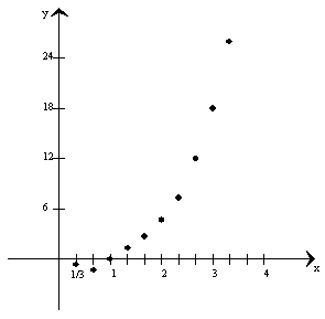
The pattern from x=1 to x=3 remains the same with f
increasing as x increases. However, from, x=0 to x=1 something new appears.
Notice how the function seems to decrease until x = 0.5, and then increases afterward.
In analyzing these different graphs (the first graph consisting of only four
points) of the same function we can state an important observation.
The behavior
of a function as reflected by its graphs is only as accurate as the number of
points plotted over the interval of interest.
That should mean if
 x were infinitely small, then the graph of the function would be the line
connecting the infinite amount of points. However, even this does not tell much. Through an
infinite number
of points we get a more and more accurate look at the functions graph or
behavior, but between any two points x and (x +
 x)
where
  x is the infinitely small distance separating the two points, there exists a
further infinite amount of points such that we cannot be sure that our graph
takes them into consideration? In other words how do we know if the graph is
continuous over the small interval separating the points? Our graph could
suddenly jump up or down as it did between x=0 and x=1.
To prove that the graph of a function is continuous over
an infinitely small interval consider a simpler function,
 An infinitely small interval implies a change in x,
 x, equal to nearly zero.
Therefore if
  is defined at any value for x,
  gives the f value of a point
located a distance
  x from x.

If the distance,  x
between the two points x and (x +
  x)
is allowed to go to zero,
what we are doing is called taking the limit
as
  x goes to a number that gets closer and closer
to zero. Mathematically this is expressed as:

Taking this limit:
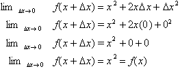
On the interval from x to x+  x
the function or y-value changes negligibly such that


This proves that points on the graph that are in between two infinitely close points
are all close to the values of the endpoints and do not jump up and down in a
random fashion. Each successive point in this interval differs from the
previous point by an amount that is related to the change in the independent
dimension. The graph is uniquely defined as a function of the independent
dimension such that for a small
 x the
x the
 f
is proportionally small.
Intuitively it is not difficult to understand why the
graph of a function is continuous over an infinitely small interval. By
definition the mathematical function expresses a relationship between
dimensions, such that one dimension is said to be dependent on the value of the
other dimension. The graph of a function reflects this relationship by relating
a horizontal change of the independent dimension with a vertical change in the
dependent dimension. Now if an imaginary function
 were to change by an
infinitely small amount then the f value would also change a similar minimal
amount, because the value of f is dependent
on the value of x.
The graph of a function is then the continuous line drawn
through an infinite set of points. For the graph to be continuous it only needs
to be defined at all points where it is being studied.
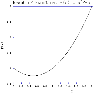
The graph of  can now be drawn as a continuous line that
corresponds exactly to the behavior of the function, f,
as the independent dimension, x, changes:
Questions
Whenever an object is thrown in the air towards some
direction, the path it follows is called a trajectory and the study of its
motion is the focus of projectile mechanics. The motion of a projectile is
dependent on several conditions such as its initial velocity when set in
motion, the angle of inclination, the force of gravity, air-resistance etc.
What makes projectile motion so interesting is that gravity only restricts the
vertical rise of the body, but has no effect on its horizontal motion parallel
to the earth’s surface. This situation gives rise to the curved trajectory or
path of the projectile.
The goal of the following problem is to find the equation
for the trajectory (graph) of a ball struck in motion by a bat at an angle of
45 degrees with an initial velocity of 50 meters per second.
The height of the ball in
motion is dependent on the horizontal distance covered and is given by the
equation:
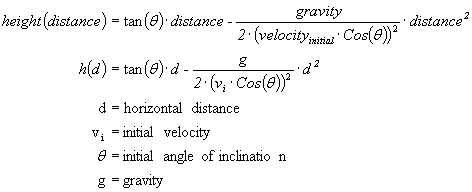
Substitute the known values for the given conditions (use g=9.8) to reduce the function to
one of two dimensions, involving vertical height as a function of horizontal
distance covered.
Get a rough idea of the graph of this projectile motion by plotting points at
intervals of  d = 1 meter. As soon as the
height is negative stop plotting.
Use
a  d=.5 m, and determine the maximum height
reached and
the distance from the firing point when it hits the ground.
Use
an angle of 60 degrees and see how the graph changes.
Double the initial velocity while using the same 45 degree initial angle of
inclination.