CHAPTER 4
Chapter 4 - The Derivative
Section 4.3 - Instantaneous Rate of Change
In this section we will take a much
closer look at rate of change and see how we can define the instantaneous rate
of change of a function at any point or value of the independent variable. Let
us begin with a study of the simple
 . Functions of the form
 , where c is a constant, express direct relationships. This
is because the value of the function, f,
is a constant multiple or fraction of the independent variable. Thus f is said
to be directly proportional to x. The
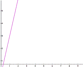
graph of the function
 looks like
From x = 1 to x = 3,
 x = 2, and
 f = 9 - 3 = 6. Thus, over this interval of
 x = 2,
 f equals 6. The average
rate at which f changed with respect
to x is by definition,
 . For each unit change in x, the change in f is 3. This tells us that f is changing three times
faster that x is changing over the
interval from x = 1 to x = 3. We can now look at the interval from x = 2 to
x = 4 where
 x equals 2.

Thus

Over this interval, the rate of
change is the same constant, 3. This leads us to conclude that the rate of
change of the function over any
interval is a constant, 3. This can be proven by the definition of rate of
change:
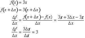
The rate of change of the direct
function
 is c and is constant
over an interval,
 x. The graph of a function
 is therefore an
increasing straight line with a constant slope or steepness equal to c. For this reason functions of the
form
 are also called linear functions since their graphs are
straight lines with a constant rate
of change.
On the other hand, the graph of the function

is not a straight
line. Unlike a line, the rate of change of

is not the same
constant over any interval
 x. To define the rate of change for the function we will have to derive a more precise way of
defining rate of change of function. To do this we will analyze the
function over small intervals of
 x
x
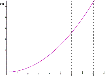
The first point to notice is that
the rate of change of the function varies with x. When x is small, f does not change that much as compared
to how much it changes when x is large. We can conclude that the rate of change
of f with respect to x, is not constant over any interval,
 x, but varies with x.
To begin our analysis let us divide
up the graph into intervals of
 = 2
and study what is happening in each of these intervals separately.
From x = 0 to x = 2,
 = 2, the change in f
is f(2) - f(0)= 4.
From x = 6 to x = 8,
 = 2, the change in f is
f(8) - f(6) = 28.
Clearly, as x
increases the rate of change of the function is increasing and is not a
constant as in our study of the line where the function changed at the same
rate as x increased.
Returning back to the graph of
 ; we calculated that from
x = 0 to x = 2 the change in f was 4.
We can then conclude that from x = 0 to x = 2 the average rate of change of the function over that particular
interval is 2 or:

Remember it is
called average because this rate of change is only valid from x = 0 to x = 2.
Now let us consider the interval
from x = 2 to x = 4 where once again the change in x,
 is 2. The change in f of the graph is equal to:
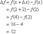
Thus the average
rate of change of the function over this interval is equal to

This value is greater than the value
we observed from x = 0 to x = 2. This implies that from x = 2 to x = 4, f(x) is
increasing at a greater rate than from x = 0 to x = 2. This is despite the fact
that in both cases the
 = 2. Therefore, the rate of change is not constant over the interval,
but is increasing
with x. When we say the rate of
change of f(x) from x = 2 to x = 4 is 6, it is only the
average value for the given interval since it assumes rate of change is constant over that interval.
Let us move on to the next interval
of x = 4 to x = 6. Once again the change in x or
 equals 2 but the corresponding change in f(x) is not
the same as before.

For x equal to 4
and  = 2, the change in the function over this interval
is

Note that this corresponds to the same value we would get by:

The average rate of change over this interval is
therefore:

This is still larger than the rate of change for the previous interval which was 6.
Remember rate of change , by definition, refers to how much the function
changes with respect to a change in
the independent variable. The steepness or slope of the line over the interval
provides a geometric understanding for this concept.
The average rate of changes
calculated over each interval can be used to approximate the graph of f(x) from x = 0 to x = 8.
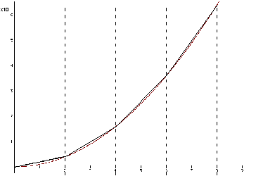
This roughly corresponds to the
original graph, but as we can see the rate of change or slope is not constant
through out the interval from x = 0 to x = 8,
but increases as x-increases. In order to get more accurate answers we need to
reduce our interval of
 =2
to a much smaller one. The idea being we need to analyze our graph over a small
interval,
  , to see what exactly is going on at each instant
the function is changing.
Here is where we begin our study of
Calculus. We break down and freeze a changing situation into an infinite series of actions and
analyzing what is going on in each individual actions.