CHAPTER 4
Chapter 4 - The Derivative
Section 4.4 - The Derivative
Calculus involves analyzing instantaneous
changes with reference to the entire system. We saw how using a small interval
of  = 2
caused great differences in the rate of change
of the function over the same interval. The function did not change nearly as much from x = 0 to x = 2
as it did from x = 4 to x = 6. The rate at which the function is changing must be dependent on the value of the function.
In other words the rate of change must be defined at each interval and this
value must be unique to that interval.
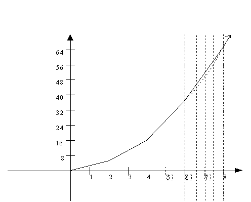
We can approximate the graph from x = 6 to x = 8 more closely by using a
smaller interval of  = 0.5.
This will give an even more accurate description of the graph of the function
 over that interval. Keep in mind that the rate of change of
the function varies with x, and the only way to accurately analyze this change
is by breaking the graph up into smaller and smaller sub-intervals and study
what is happening over these infinitely small intervals:
First let us define a method for
calculating the rate of change between any two points on the graph of f(x): If the change in f of a function from a point x to another point (x+  ) is given by:

The rate of
change of f(x) over this interval is found
by dividing by 

Remember the  on
the left side is the same as the
  in the f(x +
  )
expression.
From x = 6 to x = 6.5 the rate of change is:

From x = 6.5 to x = 7 the rate of change is:

Similarly the rate of change from x = 7 to x = 7.5 and x = 7.5 to x = 8 is 14.5
and 15.5 respectively. Notice how the
rate of change of the function slightly
increases as x increases.
This implies that there must be a way to instantaneously
define the rate of change of function through “one point” on the graph. Before continuing, take a look at how the
average rate of changes or slopes just calculated, approximate the graph from x = 6 to x = 8.

As you can see from the above graph,
the smaller interval of  = 0.5
gives a more accurate approximation of the graph of f(x). Our results are only averages
because the rate of change of f(x) is
increasing with x and is not constant
over an interval
  To define the instantaneous rate of
change, we need to define
  as an infinitely small distance separating two point x and (x+
  )
on the graph of f(x). The rate of
change calculated through these two points will then give us the exact rate of
change of f(x) at that point, x.
Since
through any one point there exists an infinite many lines, we are in actuality
giving the slope of the line through the two points x and (x+ )
where
  goes to zero. The two points are assumed to be infinitely
close to each other such that the rate of change f(x) over that interval is constant.
As we let these two points (x) and (x+  ) come closer and closer
together, the slope of the line through these two points corresponds to the
actual graph itself. For example with
  = 2, the line through x = 6 and x = 8 only roughly
represented the actual graph. However, by breaking up the interval from x = 6 to
x = 8 into four sub-intervals of
  =
1/2, we got a better approximation to the actual graph itself.
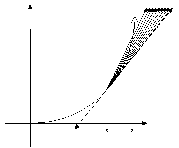
The instantaneous rate of change can
now be defined as the rate of change of the line through a point x and (x+  )
where
  is near to zero. This is called taking the limit
as
  goes to zero. In the graph this looks like.

By letting the difference or  between the two points go to zero we are able to accurately describe the
behavior of the function at any
  large we can only approximate the functions behavior over the interval. This
infinitely small
  allows us to define the rate of change of f(x) through any one point on the
graph, where point is by definition an infinitely small interval between x and
x +
 over which the rate of change is assumed to be constant or does not change.
Thus, the instantaneous rate of
change can also be thought of as the slope of the
tangent to the graph at any point.
The point is actually two simultaneous points on the graph, separated by an
infinitely small distance.
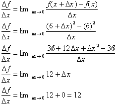
For example, the slope of the tangent to the graph
at x = 6 is given by:

We can now go on to define the rate of change at any point x
of the function
 as:
as:

This function is called the derivative and gives us the rate of
change or tangent to graph of
 at any point x. It is extremely important to
realize that the function’s derivative is also a function of x. In other words
its value changes with x to reflect a change in the rate of change of the
original function. This may sound a bit confusing but I encourage you to spend
a few minutes and think how it is so.
You are probably asking yourself how
can we assume that the derivative is constant over an infinitely small interval
 ? Since the function’s rate of change is changing then it can
only be constant over an infinitely small interval or point. It is through this
point that we define the derivative by taking the limit as
 goes to zero. In
effect we define the graph of the function through a series of connected lines
with changing slopes. In the following paragraph we will mathematically prove
that the derivatives value converges to the exact value as all errors go to
zero as
 goes to zero. Since
the graph of the function is continuous over an infinitely small interval then
so will its derivative be defined for that interval or point.
Note that  and
and
 no longer refer to discrete
values. When we let
  go
to zero, its value becomes infinitely small such that:

Here df
and dx
represent an infinitely small difference in x, where:

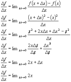
We’ll now see how to find the
derivative of any simple function,
 . Since the derivative is also a function , we shall call it f’(x), “f prime of x” where,

Our results can now be generalized
for any function
 where n is a positive integer.

From the Binomial expansion theorem we get: ( The theorem is just
algebra and you can find a proof of it by clicking here ).

This simplifies to

We can replace all the
 ,
,
 ,
with
  , which are constants:

Take note of how x goes from x to
n’th power to the 0 power while ∆x goes from the 0 power to the n’th
power in the last term. If we divide through by ∆x we get:

As we take the
limit as ∆x goes to zero, every term after the first one goes to zero and
hence cancels out; This leaves us with:

The rate of change of a function
 at any point x is
given by the function’s derivative
 evaluated at that point x.
Next section ->
Section 5.1 - Differentiating Functions